Mean Squared Error As Maximum Likelihood Estimation

14 MAR 2019 - 10 MINS

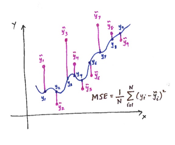
Anyone who has read about machine learning will be familiar with the Mean Squared Error (MSE) as loss function in a supervised learning model. If we generalise a bit, and think about this from a Statistics viewpoint, the MSE gives us the measure of the quality of an estimator of a parameter.

But what makes the MSE a ‘good’ measure for this? How do we define ‘good’ in this case? Hopefully this article will answer some of these questions.

Prerequisites

There is no need to understand a great deal about machine learning to make sense of this article, but it would help put things into perspective. Hopefully anyone doing a first year university course in Maths, Statistics or Computer Science shouldn’t find this too much of a stretch to read either.

It may help to be aware of the following:

• Normal Distribution
• Statistical Estimators/Models
• Maxmimum Likelihood Estimation

Defining a Statistical Model for the Data

As we said above, the main use of the MLE is to solve the problem of gauging the quality of an estimator. For this to make sense, we need to define a dataset which we can perform our calculations on.

Consider a dataset which arises from the following statistical models (A):

\[Y = g_{\theta}(X) + Z \Rightarrow^{\text{realised as}} y_i = \theta x_i + \epsilon_i\]

where \(X\) and \(Y\) are continuous random variables and we can assume the error (\(\epsilon\)) to be produced by an additive white Gaussian model¹. This implies that \(Z \sim \mathcal{N}(0, \sigma^2)\) and \(E(Z) = 0\) (B).

From a supervised learning persepctive, we will begin by observing the system which the model represents and collecting a set \(\tau = (x_i, y_i)\) for \(i = 1,...,N\) of training data, where \(x_i\)s are realisations of \(X\) and \(y_i\)s are realisations of \(Y\). The aim of the machine learning problem is to find a \(\hat{\theta}\) which best approximates \(\theta\) on the training data \(\tau\). This is done using a learning algorithm. The learning algorithm will modify \(\hat{\theta}\) based on the magnitude of the error in the approximation. This error will be given by the MSE. Once \(\hat{\theta}\) has best learned \(\tau\) (repeated the above process for all member of the training set \(\tau\) with cross validation etc.), we should have \(\hat{\theta} x_z \approx \theta x_z\), for any \(z > N\)².

Maximum Likelihood Estimate

We can define a likelihood function \(L\) involving \(\theta\) (C):

\[L(\theta) = \prod_{i=1}^N{f(Y = y_i | X = x_i, \theta)}\]

where \(f\) is the conditional probability density function of \(Y\) given input data and the learned parameter.

So by solving for the MLE of \(L\), we are expecting to get \(\hat{\theta}\); the value of \(\theta\) which maximises the likelihood of the observed data \(Y\) occurring.

Once again, from a supervised learning perspective, we can see how the likelihood function is the probability of the observed data (Y) given the parameters of the model and input data (X) = weights which have been learned (\(\theta\)).

How do we get the MSE from the MLE?

We are now at a stage where we can see how the MLE motivates the use of the MSE:

\[\begin{align} f(Y = y | X = x, \theta) & = f(Z + g(X) = y | X = x, \theta) \\ & = f(Z = y - \theta X | X = x) & \text{(sub. from A)}\\ & = f(Z = y - \theta x) & \text{(X = x)}\\ & = \frac{1}{\sigma \sqrt{2\pi}} e^{-\frac{(y-\theta x)^2)}{2\sigma^2}} &\text{(sub. from B)}\\ \end{align}\]

By finding the log-likehood function of \(C\) (\(ln L = l\)), we can keep going:

\[\begin{align} l(\theta) & = ln(\prod_{i=1}^N{f(Y = y_i | X = x_i, \theta)}) \\ & = \sum_{i=1}^N{ln(f(Y = y_i | X = x_i, \theta)}) \\ & = \sum_{i=1}^{N}ln(\frac{1}{\sigma \sqrt{2\pi}} e^{-\frac{(y_i-\theta x_i)^2}{2\sigma^2}}) \\ & = \sum_{i=1}^{N}[-\frac{1}{2}ln(2 \pi \sigma^2) - \frac{(y_i-\theta x_i)^2}{2\sigma^2}] \\ & = \sum_{i=1}^{N}[-\frac{1}{2}ln(2 \pi \sigma^2) - \frac{(y_i-\theta x_i)^2}{2\sigma^2}] \\ & = -\frac{N}{2}ln(2 \pi \sigma^2) - \sum_{i=1}^{N}\frac{(y_i-\theta x_i)^2}{2\sigma^2} \\ & = D + F \\ \end{align}\]

Since \(D\) has no \(\theta\) term in it, in order to find the \(\hat{\theta}_{} = \theta_{MLE}\), we only need to consider \(F\):

\[\begin{align} \hat{\theta} & = \text{arg}\max\limits_{\theta} (- \sum_{i=1}^{N}\frac{(y_i-\theta x_i)^2}{2\sigma^2}) \\ & = \text{arg}\min\limits_{\theta} (\sum_{i=1}^{N}{(y_i-\theta x_i)^2}) \\ & = \text{arg}\min\limits_{\theta} (\frac{1}{N} \sum_{i=1}^{N}{(y_i-\theta x_i)^2}) \\ & = \text{arg}\min\limits_{\theta} (MSE_{\tau}) \\ \end{align}\]

At this stage, by square rooting the function we are trying to minimise, we also end up with the root mean square error. Similarly other loss functions can be derived and their use justified.

Conclusion

Here we can see how by finding the \(\theta\) (weights/model) which minimses the MSE, we are in turn maximising the likelihood of getting our observed data (\(Y\)) from a given input data set (\(X\)). This is not to say that our model will generalise well to unseen input data, however given a sufficiently large dataset (and many other factors of course…) we should see an improved out of sample prediction quality also. This also highlights why the MSE (and RMSE etc.) is a mathematically logically loss function to choose.

Further Reading + References:

• The Elements of Statistical Learning (ML Bible) - Chapter 2.6
• Imperial College London, Data Science Society - Academy of AI Notes, Session 6 Slides 8-14
• Eugine Kang’s Medium Article - Maximum Likelihood Estimation
• Will Kurt’s Blog - A Deeper look at Mean Squared Error

---