Bayesian Time Series Modelling Using Facebook Prophet

05 JUL 2019 - 10 MINS

Time series analysis is known to be a particularly challenging area of data science. I would put this down to three key factors:

1. Datasets tend to be quite small. So given 10 years of weekly data for example, this boils down to only around 520 usable data points assuming the dataset is clean, well-structured and has no outlier/anomalies. From this we may need to accurately forecast a trend for the next quarter which is obviously a challenging task¹.
2. Following on from the previous point, the rate of global change is increasing. So although the historal data may suggest a certain trend, this may no longer be the case for the last 5 years. If we then try to analyse data from the last 5 years only, there may be too few data points to make any reliable predictions. An obvious example would be global climate temperature or global population growth.
3. Many factors affecting the response variable cannot be captured in the dataset. This is the case with most datasets and it is of course the job of the data scientist to engineer meaningful features to factor into the model. However, a lot of factors are circumstantial and can be near impossible to engineer e.g. factors affecting the bitcoin bubble prior to January 2018 or natural disasters which could cause an economy to collapse. New factors will also arise which were not meaningful in the context of the historical data.

With so many factors at play, data scientists need a very thorough understanding of a time-varying system to provide useful insights. As a result, clients prefer simpler, explainable model with some confidence interval then a complicated one. So although a machine learning algorithm might be better able to learn unusual trends and features, it is essentially a black-box in terms of what it has learned. A statistical model might be preferred.

Traditional time series forecasting techniques from the ARMA family of models, showcase their strengths when there are noticeable patterns in the data (i.e seasonality and stationarity trends). Information about such patterns can be used directly to create the model. However, when there is some known business trend/insight which cannot be inferred from the data, the intuition for sampling and fitting a model on a prior becomes far more evident, as the underlying trends can be Hence the need and increasing popularity of Bayesian modelling techniques.

Facebook has done a particularly good job at addressing this issue with their Prophet API. It uses a Markov Chain Monte Carlo (MCMC) sampling algorithm to fit and forecast time series data. It won’t go into the details of the algorithm here but will rather focus on the software engineers perspective of how usable the package is and how its performance compares to ARMA models and RNNs².

Facebook Prophet

Example: Temperature

The following example uses the Earth surface temperature dataset on Kaggle put together by the Berkeley Earth team.

We rename columns to Prophet’s expected format. There need to be ‘ds’ and ‘y’ columns; ‘ds’ will be in a Pandas datestamp or Pandas timestamp format and ‘y’ will be the numeric feature we want to forecast.

uk_avg_temp = pd.read_csv(...)

# Convert date strings to datetime objects.
uk_avg_temp['dt'] = pd.to_datetime(uk_avg_temp.dt)

columns = {'dt': 'ds', 'AverageTemperature': 'y'}
uk_avg_temp.rename(columns=columns, inplace=True)

We perform the train-test split and can train the out-of-the-box model on the training data.

from fbprophet import Prophet

model = Prophet()
model.fit(train)

A dataframe needs to be initialised to hold the forecasted values. The default units of a period in Prophet are days. We can change this by setting the freq argument.

# Forecast intervals will be month wise, so we set the future 
# df to being in monthly units.
future = model.make_future_dataframe(periods=len(test), freq='M')
forecast = model.predict(future)

model.plot_components(forecast)

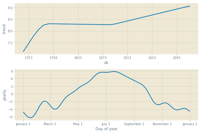
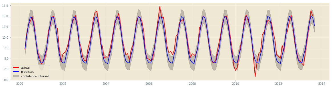
Prophet also produces an error bound under the yhat_lower and yhat_upper fields in the forecast dataframe. The expected forecast is under yhat.

plt.fill_between(forecast.ds, forecast.yhat_lower,
                 forecast.yhat_upper, color='k', 
                 alpha=.2, label='confidence interval')
plt.plot(test.index, test.AverageTemperature, color='red', 
         label='actual')
plt.plot(forecast.ds, forecast.yhat, color='blue', 
         label='predicted')
plt.legend()
plt.show()

Example: AAPL Stock Prices

In this example we examine Apple stock prices. It is almost always unreliable to use any kind of forecasting algorithm to predict for stock prices (and expect to make any money from this). Regardless, this still allows us to see Prophet’s key feature of being able to easily factor useful assumptions or heuristics into a model.

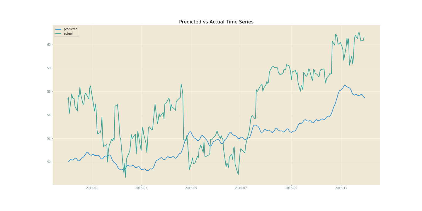
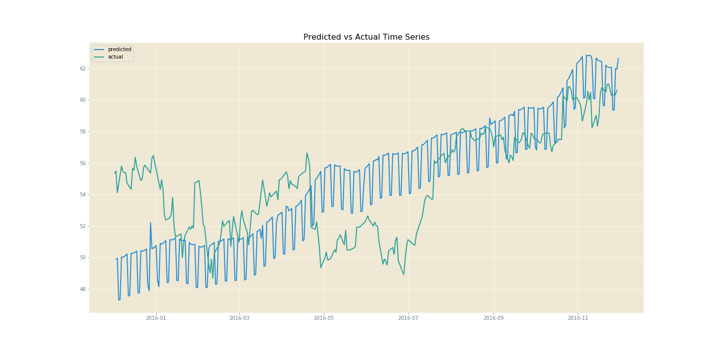
We can look at SMAPE and RSME metrics to get a sense of the model’s performance. It is also useful to look at the predicted and expected out-of-sample graph to get a sense of how successfully the trend has been learned. This is often not clear from the metrics alone.

If we run Prophet with only weekly and yearly regressors, we get the following metrics and graph. Although the magnitude of the peaks and trough in haven’t been captured very well, there is still a clear correspondance between the changepoints on both lines. This is often all that is required from time series modelling for stock prices³; an indication of when the price will go up or down, giving the user an idea of when to buy or sell.

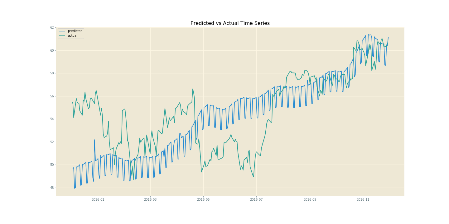
The most obvious exogenous factor that I thought would contribute to AAPL stock fluctuations would be the (potential) launch of a new product. These would be indiciated by the dates of Apple’s annual developers conference, where such announced tend to be made. So I decided to scrape a Wikipedia page for the appropriate dates and factor those into the model as changepoints, which can be done directly though Prophet’s interface. Prophet also allows you to factor regional holidays into the model, and includes regressors for each of these. There may be a spike in Apple product sales during holidays in key regions such as the UK, US and China. With more regressors we do get a spikier model, but this could easily smoothed by fitting a polynomial (np.polyfit) curve, a Fourier series or spline curves through it. Regardless, we see an increase in the performance metrics and better fitting of peaks and troughs of the original curve.

from fbprophet.make_holidays import make_holidays_df

key_dates = [scraped dates from Wikipedia page]

# Get Holiday dates from key regions that Apple sells
# its products in within the date range of all available
# time series data.
year_list = list(df.index.year.unique())
chinese_holidays = make_holidays_df(year_list=year_list, country='CN')
uk_holidays = make_holidays_df(year_list=year_list, country='UK')
us_holidays = make_holidays_df(year_list=year_list, country='US')

# Create dataframe with holiday dates in Prophet's expected format.
holidays = pd.concat([chinese_holidays, uk_holidays, us_holidays]) \
    .sort_values('ds') \
    .drop_duplicates(subset=['ds'], keep='first') \
    .reset_index() \
    .drop(columns=['index'])


model = Prophet(yearly_seasonality=11, weekly_seasonality=11, 
                changepoints=key_dates, holidays=holidays)
model.fit(train_df)

I wanted to include iPhone sales statistics as another factor to regress on, as I felt this would directly impact AAPL’s stock price, however this data was very difficult to collect. Instead I have opted for using Google search trends for the term ‘iPhone’. Hopefully this would serve as a meaningful factor when quantifying the popularity of Apple products. This resulted in slightly worse performace metrics. Although the result better fit the upward trend of the AAPL stock price, it didn’t consider the occasional dip. This may be because when Apple gets negative press, their search results may still increase although their stock price would decrease.

model = Prophet(yearly_seasonality=11, weekly_seasonality=11, 
                changepoints=key_dates, holidays=holidays)
model.add_regressor('Searches')
model.fit(train_df)

Comparison to ARIMA

It is also quite easy to factor in business knowledge in the form of other regressors into an ARIMA family model. Statsmodels allows you to factor in exogenous regressors into SARIMAX, VARIMAX and ARIMA models. However, the nature of these models means that there are many parameters which need to be tuned, often based our interpretations of Fourier transform spectral decompositions, ACF plots, PACF plots and stationarity tests. This is obviously prone to error, requires a lot of understanding to do and can be incredibly tedious.

This is not to say that using Prophet requires no understanding of the underlying mathematical concepts. Yet given the way that Facebook has packaged up this MCMC time series forecaster, one can gain familiarity with the maths through actually trying out the model with example data, since it is very easy to use out of the box, very much unlike Statsmodels’ ARIMA models.

Comparison to RNNs

With RNNs, you can configure the model for multivariate time-series inputs also. However the main issue here is with training times due to the large matrix of weights that the model is learning. After being tuned, RNNs can produce highly accurate models which often overfit the data, which also begs the question as to whether all the learned information is actually necesary. For a stock price forecast, a general idea of which direction the price will move in within some degree of uncertainty and magnitude of fluctuation is sufficient. This can be done using statistical methods with far less computational effort than a machine learning model, and Prophet makes this particularly easy. Since model in production are often retrained as new data becomes available, statistical models can lead to significant performance improvements.

More general issues also arise with explainability when using machine learning models over statistical ones ⁴.

TL;DR

• Prophet is easier to use for non-experts than RNNs and ARIMA models; allows you to easily factor in business understanding and intuition through exogenous regressors.
• Requires significantly less training time and parameterisation effort than alternative models.
• Prophet is a great untuned baseline for univariate and multivariate time series modelling problem.

As I have stated a few times, for financial time series modelling we only really need to know whether the prices will go up or down and some degree of uncertainty or magnitude of the fluctuation. With this is mind, we can use a standard scaler, which centers all data points around 0, and a log scaler to remove any skew, and then pass the time series through the same models. This will generally give you more meanignful insights and better metrics, although this is out of the scope of this article. I have included feature scaling, feature engineering, such as the code used to scrape the web, other time series models, such as RNNs and SARIMAX, and all other code used to produce the graph above in this Jupyter notebook.

Further Reading + References:

• Challenges to Time Series Analysis in the Computer Age by Clifford Lame from LSE

• Sorry ARIMA, but I’m Going Bayesian from Kim Larsen’s blog
• 7 Ways Time Series Forecasting Differs from Machine Learning from Oracle’s data science blog
• Facebook Prophet Docs